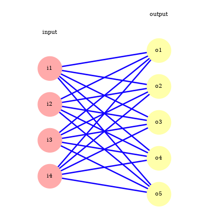
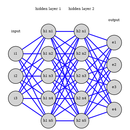
Neural network training
Feedforward step
Training the neural network
A neural network is trained through back-propagation. It allows to adapt the weights in the layer successively.
Moving from the perceptron to a continuous activation function allows this.
The idea is to start from the end of the network and evaluate the difference between the output of the network and the target from the training set.
We use this as the error for the last layer. We also propagate the error to the last hidden layer and adapt the weights between the last and second-to-last layer accordingly.
Last layer
The last layer is slightly different so we treat it first.
Let's look at the last set of parameters between the output and the hidden layer.
We have the loss function
$$ J = -\sum_{i,j} y^{(i)}_{j} \log(\hat y^{(i)}_{j})$$where $y^{(i)}_{j}$ is 1 if training sample $i$ is in class $j$, 0 otherwise.
$\hat y^{(i)}_{j}$ is the prediction of the model, here
$$ \hat y^{(i)}_{j} = s_j(z_j^{(i)} )$$with $z_j^{(i)}$ the linear combination of the last hidden layer with the last set of coefficients $w_{jk}$.
We can calculate the derivative of the loss function with respect to the linear combination in the last layer:
$$ \frac{\partial J}{\partial z_j^{(i)}} = \sum\limits_{l=1}^{n_o}\frac{\partial J}{\partial \hat y^{(i)}_{l}} \frac{\partial \hat y^{(i)}_{l}}{\partial z_j^{(i)}} = \sum\limits_{l=1}^{n_o} \left( -\frac{y^{(i)}_{l} }{ \hat y^{(i)}_{l} }\right) s_l\left(\delta_{lj}-s_j\right) $$with $n_o$ the number of units in the output layer.
$$ \frac{\partial J}{\partial w_{km}} = \sum\limits_{i=1}^{n_d}\sum\limits_{j=1}^{n_o}\frac{\partial J}{\partial z_j^{(i)}}\frac{\partial z_j^{(i)}}{\partial w_{km}} = \sum\limits_{i=1}^{n_d}\sum\limits_{j=1}^{n_o} \sum\limits_{l=1}^{n_o} \left( -\frac{y^{(i)}_{l} }{ \hat y^{(i)}_{l} }\right) s_l\left(\delta_{lj}-s_j\right) \frac{\partial z_j^{(i)}}{\partial w_{km}} $$with
$$ \frac{\partial z_j^{(i)}}{\partial w_{km}} = x^{(i)}_k \delta_{mj}$$we get
$$ \frac{\partial J}{\partial w_{km}} = \sum\limits_{i=1}^{n_d} \sum\limits_{l=1}^{n_o} \left( -\frac{y^{(i)}_{l} }{ \hat y^{(i)}_{l} }\right) s_l\left(\delta_{lm}-s_m\right) x^{(i)}_{k} $$Layer error treatment
We now look at a standard layer.
Now we can consider a normal layer with sigmoid activation with input $x$, parameters $w$ and output $y$. We denote with $z$ the linear combination of $x$ that enters the activation function (the sigmoid function).
$$ y_j = \phi(z_j) $$$$ z = W^T x $$We have $$ \frac{\partial y_j}{\partial z_{j}} = y_j(1-y_j)$$ and $$\frac{\partial y_j}{\partial w_{ij}} = \frac{\partial y_j}{\partial z_{j}} \frac{\partial z_j}{\partial w_{ij}} = \frac{\partial y_j}{\partial z_{j}} x_i = y_j(1-y_j) x_i$$
We can now calculate the derivative of the loss function with respect to the parameters of the connections:
We see that the derivative depends on the gradient of the loss with respect to the outputs of the layer we are considering. This output is the input into the next layer. So it will be useful to be able calculate the derivative of $J$ with respect to the layer input.
with
$$ \frac{\partial J}{\partial z_{j}} = \frac{\partial J}{\partial y_{j}} \frac{\partial y_j}{\partial z_{j}} = \frac{\partial J}{\partial y_{j}} y_j(1-y_j) $$To adapt the parameters of the network we start with the last layer and do for each layer:
- calculate the derivatives with respect to the outputs to adapt the weights
- calculate the derivatives with respect to the inputs to use in the calculation of the parameters of the previous layer.
The parameter adaptation goes in the opposite direction as the prediction, it is called back-propagation.
Initial weights
We need to break the symmetry between nodes at initialisation time otherwise all nodes will be updated together.
Difficulties with network training
Training a neural network is challenging because:
- the loss function is not convex (there are local minima)
- if weights get too large the argument of the sigmoid activation gets large, which means the derivative get small and convergence is very slow.
- neural network are prone to overfitting
Regularisation
Neural networks have many parameters and can easily overfit. To prevent it there are several options:
- reduce size of the network
- early stopping: do not allow the network to optimize its weights until a minimum is found
- add random noise to the weights or to the units activities
- add a penalty for large weights as we did for other algorithms